Fine-Tuning NLP Models With Hugging Face

Part 1: Getting Started

Kedion

14 min readSep 21, 2021

Written by Tigran Avetisyan

This is Part 1 of our 3 PART SERIES on Hugging Face.

See Part 2 here.

NLP and Language Models
What Is Hugging Face?
The Hugging Face Inference API
Batch inference with the Inference API
Using Transformers Pipelines
Getting Started With Direct Model Use

NLP and Language Models

Natural language processing, or NLP, is an exciting field that has seen dramatic development in recent years. Today, language models like GPT-3 (Generative Pre-trained Transformer 3) can produce text that is indistinguishable from that written by a human, which is sensational from a technological standpoint but controversial when we are talking about ethics.

You can easily build and train quality NLP models right on your computer as well (though you probably won’t be reaching GPT-3 levels of convincingness). However, starting with NLP can be tricky because of data requirements and preprocessing rules for text sequences.

If you want to make use of natural language processing right now, you could leverage an NLP framework like Hugging Face, which is an API that facilitates the use of language models for large-scale inference.

In this guide, we are going to introduce you to the features and capabilities of Hugging Face, and we will also showcase the basics of inference with pretrained Hugging Face models.

Let’s get started!

What Is Hugging Face?

Hugging Face is a community and NLP platform that provides users with access to a wealth of tooling to help them accelerate language-related workflows. The framework contains thousands of models and datasets to enable data scientists and machine learning engineers alike to tackle tasks such as text classification, text translation, text summarization, question answering, or automatic speech recognition.

*The models available in Hugging Face, organized their* ***goal***.

In a nutshell, the framework contains the following important components (there are more):

The Transformers library. Transformers allows you to leverage the models and datasets provided by Hugging Face. Note that the library requires that you have either TensorFlow 2.x.x or PyTorch installed.
Inference API. With the Inference API, you may perform prediction via HTTP requests with only minimal code. The Inference API relies on pretrained models.
Pretrained transformer models. Hugging Face provides access to over 15,000 models like BERT, DistilBERT, GPT2, or T5, to name a few.
Language datasets. In addition to models, Hugging Face offers over 1,300 datasets for applications such as translation, sentiment classification, or named entity recognition.

The Hugging Face Inference API

The Inference API is the key component of Hugging Face and is the one that will interest most potential users of the framework. Hugging Face has built the API for those who are not willing or are not technically adept enough to delve into code and those who want to get started with their projects in a short timeframe. Additionally, since the Inference API is hosted in the cloud, you don’t have to deploy any models in your local environment.

To start using the Inference API, you need to sign up with Hugging Face. The platform offers a number of subscription plans — a free plan with limited features and several paid plans with increased API request limits and access to accelerated inference.

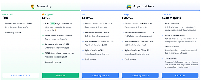
The free plan is perfectly sufficient for testing out the Inference API. If you end up liking the framework, you may upgrade to a paid plan in accordance with your project’s needs.

Performing Inference with the Inference API

— — Building a query function — —

To leverage the Inference API, you simply need to craft an HTTP request as follows:

Above, we defined a function to perform a query to the Inference API. The Inference API requires that you pass the following arguments:

model_id — the ID of the model you want to use to process the payload.
payload — the text data you want to perform operations on.
api_token — the token of your Hugging Face account. Your API token allows Hugging Face to determine which API features you have access to based on your subscription plan.

The function returns a response in JSON format (though you may freely manipulate the results in whichever way you see fit for your needs).

The model_id argument determines which model will be used to carry out your requests. To locate model_id, you should choose a model from the Hugging Face model directory and copy the endpoint at the very top of the webpage. As an example, if we take the RoBERTa base SQuAD model, here’s what the endpoint looks like:

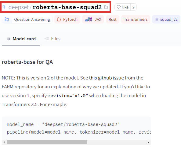
RoBERTa base SQuAD is a model built to answer questions based on an input question and provided context for the answer. The model choice in this example is arbitrary — for real-world applications, you would select a model based on your goals.

Next, we need to define our payload. The payload needs to conform to the input format of the selected model, which you can find under Usage down the webpage of your respective model.

In the case of RoBERTa base SQuAD (and other question answering models), input data is a dictionary with two keys and associated sequences:

Question — the question you want the model to answer.
Context — the context the model will use to generate an answer.

Lastly, we have the API key. Assuming you’ve set up an account on Hugging Face, you will find your API key at https://huggingface.co/settings/token.

Single-question requests with the Inference API

Here’s how we put the code together and make a request to the Inference API:

Our response is a dictionary with the following contents:

{'score': 0.9129266142845154, 'start': 9, 'end': 15, 'answer': 'Monday'}

Here:

score represents the confidence of the model in its output.
start shows the start index of the answer in the provided context.
end shows the end index of the answer in the provided context.
answer is simply the answer to our query.

Batch inference with the Inference API

You don’t have to feed input sequences one-by-one — you can perform batch prediction by just stuffing your input dictionaries in a Python list (or any other container of your choice):

For this query, the response would be as follows:

[{'score': 0.9129266142845154, 'start': 9, 'end': 15, 'answer': 'Monday'}, {'score': 0.9501503705978394, 'start': 31, 'end': 35, 'answer': '1980'}]

From this example, we not only got to see the Inference API in action, but we also saw that the RoBERTa base SQuAD model can accurately answer our questions based on context!

Performing Invalid Requests With The Inference API

To conclude this section, let’s demonstrate what happens if your query request fails (e.g. if your input data format is wrong). Note the key “text” instead of “context” in the input dictionaries.

The response to this query would be as follows:

{'error': 'unknown error', 'warnings': ["'You need to provide a dictionary with keys {question:..., context:...}'"]}

The Inference API doesn’t throw any exceptions — instead, whenever anything goes wrong, error messages will be delivered to you in the response.

These have been the basics of using the Inference API. Play around with the code yourself to find out what it can do for you!

Pipeline VS Direct Model Use In Inference

The Inference API completely abstracts the “behind the scenes” aspects of inference, which is great if you want to start using NLP models quickly. But if you would like to get direct access to the models for fine-tuning or just for self-learning purposes, you should use the Transformers library.

Transformers can be installed with pip:

Or with Conda:

There are more ways to install Transformers — check out the library’s installation guide to learn more.

Transformers allows you to run inference and training on your local machine. Once you get Transformers installed on your machine, you will get access to two primary ways to do inference and/or training:

Via pipelines.
Via direct model use.

Let’s have a look at each of these methods below!

Using Transformers Pipelines

Similar to the Inference API, pipelines hide away the process of inference, allowing you to get predictions with just a few lines of code.

Pipeline instantiation is done as follows:

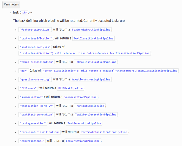
The pipeline method has only one mandatory parameter — task. The value passed to this parameter determines which pipeline will be returned. The following pipelines are available for selection:

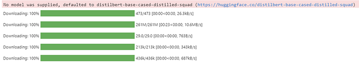
Optionally, you may also specify a pre-trained model and tokenizer to be used. If you don’t provide these arguments, the pipeline will load the default model for the specified task and the default tokenizer for the specified model.

In our case, the default model is DistilBert base cased distilled SQuAD.

To keep things simple, we’ve again selected “question-answering” for our pipeline.

Note that if you request a model and tokenizer pair for the first time, Transformers will need to download the files onto your machine. Downloaded files are cached for reuse.

You may also set up Transformers to work in a completely offline environment, but this is beyond the scope of this post. The installation guide of Transformers contains more information about offline use.

Anyway, once we’ve got our pipeline loaded, we may directly proceed to inference. To do this, we just pass a query to the pipeline, like so:

[{'score': 0.9574882984161377, 'start': 9, 'end': 15, 'answer': 'Monday'}, {'score': 0.9639834761619568, 'start': 31, 'end': 35, 'answer': '1980'}]

As you can see, carrying out inference with pipelines is very similar to how you use the Inference API. However, pipelines are hosted on your local machine (rather than in the cloud), and their setup process is somewhat different.

Using Pre-trained Transformers Models Directly

If you want to customize your code even further, you could access pre-trained Transformers models directly.

Transformers offers models in TensorFlow and/or PyTorch. The model usage process is very similar in either of the libraries, but there are some subtle differences in the code. You should consult Transformers’ “Summary of the tasks” for more information about implementation details.

We will be using TensorFlow to showcase direct model use. And once again, we will stick to the task of question answering to keep this section consistent with the previous ones.

Getting Started With Direct Model Use

To get started with direct model use, we need to import two classes:

AutoTokenizer — a class that we will use to automatically instantiate a pre-trained tokenizer.
TFAutoModelForQuestionAnswering — a class that will help us automatically obtain the weights of a TensorFlow model for question answering. The equivalent class for PyTorch is AutoModelForQuestionAnswering.

You can find more information about available auto classes (for tokenizers and model loaders) in the Transformers documentation.

And here’s how we instantiate our tokenizer and model:

To obtain a pretrained tokenizer and model, we use the from_pretrained method with both classes, supplying the ID of the associated model. Instead of the ID, you may also supply a path or URL to a saved vocabulary file or model weights.

Here, note the use of the from_pt parameter. The RoBERTa base SQuAD model we have been using throughout this guide is built with PyTorch, and no “native” TensorFlow models are available (as of this post’s writing). However, the from_pt parameter allows us to convert PyTorch models to TensorFlow. This works the other way around as well through the from_tf parameter in PyTorch auto models.

With all that said, keep in mind that conversion may not always be smooth. In the case of RoBERTa base SQuAD, we’ve got the following warning:

So not all of the weights of the pre-trained PyTorch model were carried over to the TensorFlow model. This won’t matter now since we are only going to show how to use Transformers models rather than how to achieve great results with them.

Tokenizing Question-Context Pairs

To perform inference with the loaded model, we need to tokenize our question and its corresponding context as follows:

When calling the tokenizer, we do the following:

Provide our question via the text parameter and our context via the text_pair parameter.
Set the add_special_tokens parameter to True so that the tokenizer separates our question and context with special tokens. This is necessary because the tokenizer joins the input question and context into one string.
Pass “tf” to the return_tensors argument so that we get the input as a TF Tensor.

Note that depending on your model, you may need to make use of the other parameters of the tokenizer (such as maximum input length). You can find out more about some tokenizer parameters here.

Here’s what the inputs variable contains, if you are curious:

{ "input_ids": < tf.Tensor: shape = (1, 20), dtype = int32, numpy = array([[0, 1779, 21, 38, 2421, 116, 2, 2, 100, 21, 2421, 11, 2921, 6, 2805, 6, 11, 5114, 4, 2]])> , "attention_mask": < tf.Tensor: shape = (1, 20), dtype = int32, numpy = array([[1, 1, 1, 1, 1, 1, 1, 1, 1, 1, 1, 1, 1, 1, 1, 1, 1, 1, 1, 1]]) >}

As we can see, the inputs variable contains inputs_ids, which are the tokens assigned to our input question and context. Additionally, inputs contains an attention mask that, in our case, assigns equal importance to our inputs.

In the code block above, we’ve extracted the input IDs from the tokenized object and assigned them to the input_ids variable. Let’s see what it contains:

[0 1779   21   38 2421  116    2    2  100   21 2421   11 2921    6
2805    6   11 5114    4    2]

If we converted the input_ids back to a string, we would get the following:

<s>When was I born?</s></s>I was born in Detroit, USA, in 1980.</s>

This shows us that the tokenizer combined our question and context and indicated their beginning and end with a special token to let the model know which is which. Without these tokens, the model would not be able to accurately answer our questions.

Performing Single-Sample Inference With Direct Model Use

Now, let’s feed our inputs into the model and examine the outputs:

TFQuestionAnsweringModelOutput(loss = None, start_logits = < tf.Tensor: shape = (1, 20), dtype = float32, numpy = array([   [1.2259467, -7.791437, -8.260778, -8.249651, -7.5693817,    -7.936594, -8.363062, -7.1329803, -0.18496554, -2.9790633,    -1.8434091, -1.3693225, 0.71017456, -5.1979237, -1.2315122,    -4.5270185, 0.62987506, 6.598527, -1.2783077, -7.465865   ]  ],  dtype = float32) > , end_logits = < tf.Tensor: shape = (1, 20), dtype = float32, numpy = array([   [1.6835405, -6.918748, -7.306207, -7.5368285, -6.0764575,    -3.6980824, -5.6374154, -4.4059825, -4.577457, -5.964948,    -2.6135447, -5.8583727, -0.7394024, -5.670526, 0.16733687,    -2.0341313, -2.189781, 7.048407, 3.6379344, -4.67701   ]  ],  dtype = float32) > , hidden_states = None, attentions = None)

The model output contains two TF Tensors — start_logits and end_logits. Essentially, these Tensors show the positions in the input at which the model thinks the answer to the input question starts and ends.

To be able to pinpoint the exact position of the answer, we need to locate the indices with the maximum scores, like so:

Notice that with answer_end, we add 1 to the index with the maximum score. This is to ensure that we don’t lose the last word in the answer after we slice the input sequence.

Let’s see the values for answer_start and answer_end:

Answer start index: 17
Answer end index: 18

And to retrieve our answer, we need to convert the IDs between the start and end indices back to a string:

Answer to the question:  1980

Notice that the output contains a space before “1980”. We won’t bother removing it in this guide, but you could easily do so if necessary.

In this particular example, the model picked one word — 1980 — as the answer to our question. But it can output answers with several consecutive words as well, which we can see if we rephrase the question to “Where was I born?”

Answer start index: 12
Answer end index: 15
Answer to the question:  Detroit, USA

Performing Batch Inference With Direct Model Use

The examples above showed how to process a single-sample query. For batches of questions, one option would be to iterate over the questions & contexts and predict an answer for each of them separately:

Question: Where was I born?
Context: I was born in Detroit, USA, in 1980.
Answer start index: 12
Answer end index: 15
Answer to the question:  Detroit, USA

Question: What day is it?
Context: Today is Monday.
Answer start index: 10
Answer end index: 11
Answer to the question:  Monday

Alternatively (and more optimally), we can vectorize the inference of question answers. Let’s see this in action using the questions and contexts from the previous example:

Notice the new parameter padding. We need to use this parameter whenever our input sequences have unequal length. When padding is True, the tokenizer will pad all sequences to make them as long as the longest sequence in the input.

Next, we pass our inputs to the model and extract the input IDs from our inputs Tensor:

Let’s inspect input_ids to figure out how they are different from the IDs with single-sample inference:

[[    0 13841    21    38  2421   116     2     2   100    21  2421    11    2921     6  2805     6    11  5114     4     2]  [    0  2264   183    16    24   116     2     2  5625    16   302     4       2     1     1     1     1     1     1     1]]

inputs_ids contains two NumPy arrays — one for each input question-context pair. Let’s convert the second array back to a string to see its contents:

<s>What day is it?</s></s>Today is Monday.</s><pad><pad><pad><pad><pad><pad><pad>

This is indeed our second question-context pair! We can also see how the tokenizer handled its padding.

Next, let’s have a look at the output of our model:

TFQuestionAnsweringModelOutput(loss=None, start_logits=<tf.Tensor: shape=(2, 20), dtype=float32, numpy= array([[ 0.78155375, -8.073274  , -8.34409   , -8.468487  , -8.099401  ,         -8.646169  , -8.6963625 , -7.6574035 , -0.64569664, -3.0957458 ,         -2.2456067 ,  0.14127505,  6.086786  , -3.696553  , -0.37048122,         -5.0749235 , -2.5687819 ,  0.3333048 , -3.133765  , -8.028114  ],        [ 1.7058821 , -8.217684  , -8.914576  , -8.764219  , -8.871216  ,         -9.367665  , -9.4340925 , -8.613971  , -0.7869898 , -5.4473844 ,          5.1352215 , -4.5842705 , -8.896799  , -9.427734  , -9.427734  ,         -9.427734  , -9.427734  , -9.427734  , -9.427734  , -9.427734  ]],       dtype=float32)>, end_logits=<tf.Tensor: shape=(2, 20), dtype=float32, numpy= array([[ 1.0022359 , -7.5837913 , -7.652511  , -7.7337627 , -6.577329  ,         -4.721192  , -6.1436515 , -4.644155  , -5.339603  , -6.4877644 ,         -3.6098654 , -3.8038702 ,  5.0979486 , -1.4663633 ,  5.515522  ,          1.7955147 , -4.917917  ,  2.0246046 ,  2.1283152 , -5.46772   ],        [ 1.9663267 , -7.624847  , -5.9132714 , -7.2117314 , -7.2619796 ,         -6.2353854 , -6.845627  , -7.1807027 , -3.6652987 , -6.841409  ,          4.9925647 ,  0.33412167, -7.2172003 , -8.610821  , -8.610821  ,         -8.610821  , -8.610821  , -8.610821  , -8.610821  , -8.610821  ]],       dtype=float32)>, hidden_states=None, attentions=None)

The start_logits and end_logits Tensors are each composed of two arrays that correspond to our question-context pairs.

Next, let’s retrieve the indices with the highest scores:

Here’s what we get:

Answer start indices: [12 10]
Answer end indices: [15 11]

Now, let’s use the indices to retrieve our answers:

And here’s the result:

[' Detroit, USA', ' Monday']

And to put it all together and make sure that the answers correspond to our questions, we can do the following:

Question 1: Where was I born?
Context 1: I was born in Detroit, USA, in 1980.
Answer start index: 12
Answer end index: 15
Answer 1:  Detroit, USA

Question 2: What day is it?
Context 2: Today is Monday.
Answer start index: 10
Answer end index: 11
Answer 2:  Monday

The answers indeed match our questions, so we’ve done everything correctly!

Next Steps

And this concludes our guide for inference via direct model use with Hugging Face — for now!

The usage of other Hugging Face models in other tasks will be similar — however, you will need to check:

The expected input format of your model.
How to tokenize input sequences for your specific application.
How to interpret model outputs and how to convert tokenized sequences back into string form.

The basics of direct model use with Hugging Face are described in the documentation of Transformers, so make sure to check it out!

Note that the documentation doesn’t go into much detail about certain aspects of Transformers. Often, you will need to figure out model input formats on your own, and you’ll also need to figure out how to interpret outputs. But this is part of the learning experience!

That’s it!

We covered a lot in this article. Now check out Part 2, where we learn to fine-tune NLP models with Hugging Face.

Code

You can find all code for this article in the Jupyter notebook here.